

How To Draw A Sample Distribution
vi.ii: The Sampling Distribution of the Sample Hateful
- Page ID
- 570
Learning Objectives
- To learn what the sampling distribution of \(\overline{Ten}\) is when the sample size is large.
- To learn what the sampling distribution of \(\overline{X}\) is when the population is normal.
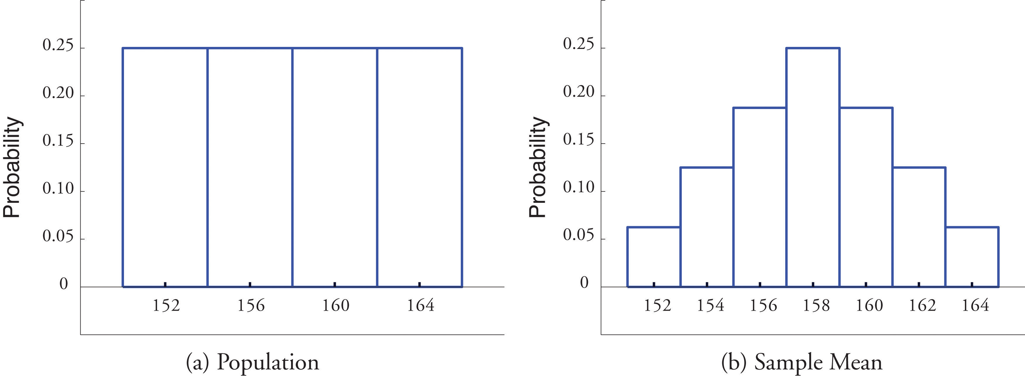
In Example half-dozen.1.i, we constructed the probability distribution of the sample hateful for samples of size two fatigued from the population of 4 rowers. The probability distribution is:
\[\begin{array}{c|c c c c c c c} \bar{x} & 152 & 154 & 156 & 158 & 160 & 162 & 164\\ \hline P(\bar{10}) &\dfrac{one}{16} &\dfrac{ii}{xvi} &\dfrac{3}{16} &\dfrac{four}{16} &\dfrac{three}{16} &\dfrac{2}{16} &\dfrac{i}{16}\\ \end{array}\]
Figure \(\PageIndex{1}\) shows a side-by-side comparison of a histogram for the original population and a histogram for this distribution. Whereas the distribution of the population is compatible, the sampling distribution of the mean has a shape approaching the shape of the familiar bong curve. This miracle of the sampling distribution of the mean taking on a bell shape even though the population distribution is not bell-shaped happens in general. Here is a somewhat more realistic example.
Suppose we accept samples of size \(1\), \(5\), \(10\), or \(xx\) from a population that consists entirely of the numbers \(0\) and \(1\), one-half the population \(0\), half \(1\), and then that the population mean is \(0.5\). The sampling distributions are:
\(n = 1\):
\[\begin{array}{c|c c } \bar{x} & 0 & i \\ \hline P(\bar{ten}) &0.5 &0.five \\ \end{array} \nonumber\]
\(n = 5\):
\[\brainstorm{array}{c|c c c c c c} \bar{ten} & 0 & 0.2 & 0.4 & 0.6 & 0.8 & 1 \\ \hline P(\bar{10}) &0.03 &0.sixteen &0.31 &0.31 &0.16 &0.03 \\ \stop{assortment} \nonumber\]
\(due north = 10\):
\[\begin{assortment}{c|c c c c c c c c c c c} \bar{x} & 0 & 0.ane & 0.2 & 0.3 & 0.4 & 0.five & 0.6 & 0.7 & 0.8 & 0.9 & 1 \\ \hline P(\bar{ten}) &0.00 &0.01 &0.04 &0.12 &0.21 &0.25 &0.21 &0.12 &0.04 &0.01 &0.00 \\ \end{array} \nonumber\]
\(n = xx\):
\[\begin{array}{c|c c c c c c c c c c c} \bar{x} & 0 & 0.05 & 0.10 & 0.15 & 0.20 & 0.25 & 0.30 & 0.35 & 0.40 & 0.45 & 0.50 \\ \hline P(\bar{x}) &0.00 &0.00 &0.00 &0.00 &0.00 &0.01 &0.04 &0.07 &0.12 &0.16 &0.xviii \\ \stop{array} \nonumber\]
and
\[\brainstorm{array}{c|c c c c c c c c c c } \bar{x} & 0.55 & 0.60 & 0.65 & 0.70 & 0.75 & 0.fourscore & 0.85 & 0.90 & 0.95 & 1 \\ \hline P(\bar{x}) &0.16 &0.12 &0.07 &0.04 &0.01 &0.00 &0.00 &0.00 &0.00 &0.00 \\ \end{assortment} \nonumber\]
Histograms illustrating these distributions are shown in Effigy \(\PageIndex{2}\).
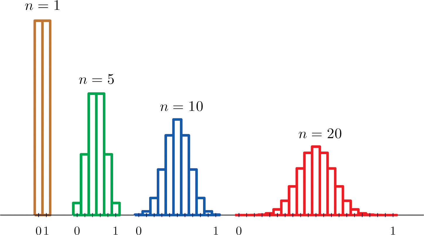
As \(n\) increases the sampling distribution of \(\overline{X}\) evolves in an interesting fashion: the probabilities on the lower and the upper ends shrink and the probabilities in the middle become larger in relation to them. If we were to proceed to increase \(n\) so the shape of the sampling distribution would go smoother and more bell-shaped.
What we are seeing in these examples does not depend on the particular population distributions involved. In full general, ane may start with any distribution and the sampling distribution of the sample hateful will increasingly resemble the bell-shaped normal bend equally the sample size increases. This is the content of the Central Limit Theorem.
The Key Limit Theorem
For samples of size \(xxx\) or more than, the sample mean is approximately normally distributed, with hateful \(\mu _{\overline{X}}=\mu\) and standard deviation \(\sigma _{\overline{Ten}}=\dfrac{\sigma }{\sqrt{n}}\), where \(n\) is the sample size. The larger the sample size, the better the approximation. The Key Limit Theorem is illustrated for several common population distributions in Figure \(\PageIndex{three}\).
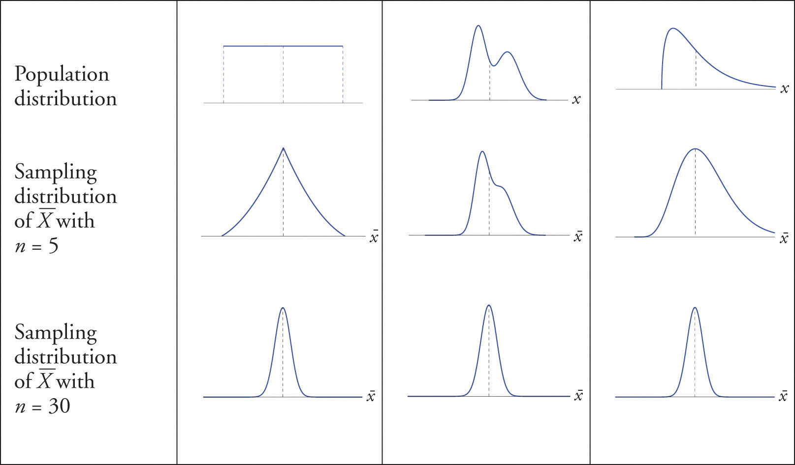
The dashed vertical lines in the figures locate the population hateful. Regardless of the distribution of the population, every bit the sample size is increased the shape of the sampling distribution of the sample mean becomes increasingly bell-shaped, centered on the population hateful. Typically past the time the sample size is \(30\) the distribution of the sample hateful is practically the same as a normal distribution.
The importance of the Central Limit Theorem is that information technology allows u.s.a. to brand probability statements about the sample mean, specifically in relation to its value in comparison to the population hateful, as we will see in the examples. But to use the consequence properly nosotros must first realize that there are two split random variables (and therefore two probability distributions) at play:
- \(X\), the measurement of a single chemical element selected at random from the population; the distribution of \(10\) is the distribution of the population, with mean the population hateful \(\mu\) and standard deviation the population standard difference \(\sigma\);
- \(\overline{X}\), the mean of the measurements in a sample of size \(n\); the distribution of \(\overline{X}\) is its sampling distribution, with mean \(\mu _{\overline{10}}=\mu\) and standard difference \(\sigma _{\overline{X}}=\dfrac{\sigma }{\sqrt{n}}\).
Case \(\PageIndex{i}\)
Let \(\overline{X}\) be the mean of a random sample of size \(50\) drawn from a population with mean \(112\) and standard divergence \(xl\).
- Find the mean and standard deviation of \(\overline{X}\).
- Find the probability that \(\overline{X}\) assumes a value between \(110\) and \(114\).
- Find the probability that \(\overline{X}\) assumes a value greater than \(113\).
Solution:
- By the formulas in the previous section \[\mu _{\overline{Ten}}=\mu=112 \nonumber\] and \[ \sigma_{\overline{X}}=\dfrac{\sigma}{\sqrt{n}}=\dfrac{twoscore} {\sqrt{fifty}}=5.65685 \nonumber\]
- Since the sample size is at least \(30\), the Central Limit Theorem applies: \(\overline{X}\) is approximately usually distributed. We compute probabilities using Effigy 5.iii.1 in the usual way, just being careful to employ \(\sigma _{\overline{X}}\) and not \(\sigma\) when nosotros standardize:
\[\begin{align*} P(110<\overline{X}<114)&= P\left ( \dfrac{110-\mu _{\overline{Ten}}}{\sigma _{\overline{Ten}}} <Z<\dfrac{114-\mu _{\overline{X}}}{\sigma _{\overline{X}}}\right )\\[4pt] &= P\left ( \dfrac{110-112}{five.65685} <Z<\dfrac{114-112}{5.65685}\right )\\[4pt] &= P(-0.35<Z<0.35)\\[4pt] &= 0.6368-0.3632\\[4pt] &= 0.2736 \end{align*}\]
- Similarly
\[\begin{align*} P(\overline{X}> 113)&= P\left ( Z>\dfrac{113-\mu _{\overline{X}}}{\sigma _{\overline{X}}}\correct )\\[4pt] &= P\left ( Z>\dfrac{113-112}{5.65685}\correct )\\[4pt] &= P(Z>0.xviii)\\[4pt] &= one-P(Z<0.18)\\[4pt] &= 1-0.5714\\[4pt] &= 0.4286 \end{align*}\]
Note that if in the higher up example nosotros had been asked to compute the probability that the value of a unmarried randomly selected element of the population exceeds \(113\), that is, to compute the number \(P(X>113)\), we would not have been able to do so, since we do not know the distribution of \(X\), only just that its hateful is \(112\) and its standard departure is \(forty\). By contrast we could compute \(P(\overline{X}>113)\) even without complete knowledge of the distribution of \(Ten\) because the Central Limit Theorem guarantees that \(\overline{X}\) is approximately normal.
Example \(\PageIndex{2}\)
The numerical population of form signal averages at a college has hateful \(two.61\) and standard deviation \(0.5\). If a random sample of size \(100\) is taken from the population, what is the probability that the sample mean will be betwixt \(2.51\) and \(two.71\)?
Solution:
The sample mean \(\overline{X}\) has mean \(\mu _{\overline{10}}=\mu =ii.61\) and standard deviation \(\sigma _{\overline{X}}=\dfrac{\sigma }{\sqrt{n}}=\dfrac{0.5}{10}=0.05\), then
\[\brainstorm{align*} P(two.51<\overline{Ten}<2.71)&= P\left ( \dfrac{2.51-\mu _{\overline{Ten}}}{\sigma _{\overline{X}}} <Z<\dfrac{2.71-\mu _{\overline{X}}}{\sigma _{\overline{Ten}}}\right )\\[4pt] &= P\left ( \dfrac{2.51-2.61}{0.05} <Z<\dfrac{2.71-2.61}{0.05}\right )\\[4pt] &= P(-2<Z<ii)\\[4pt] &= P(Z<2)-P(Z<-two)\\[4pt] &= 0.9772-0.0228\\[4pt] &= 0.9544 \stop{align*}\]
Usually Distributed Populations
The Cardinal Limit Theorem says that no affair what the distribution of the population is, every bit long as the sample is "large," pregnant of size \(30\) or more than, the sample mean is approximately normally distributed. If the population is normal to brainstorm with so the sample mean also has a normal distribution, regardless of the sample size.
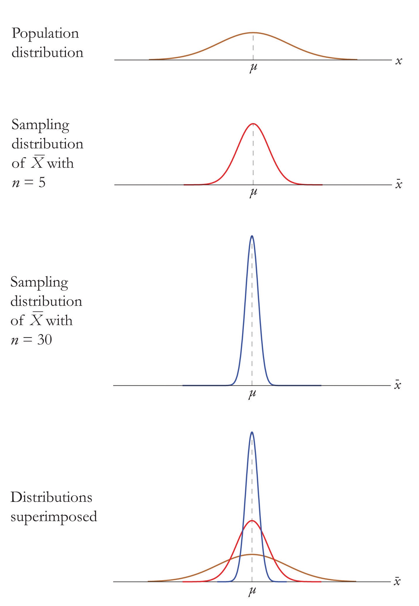
For samples of whatsoever size fatigued from a usually distributed population, the sample mean is normally distributed, with mean \(μ_X=μ\) and standard deviation \(σ_X =σ/\sqrt{due north}\), where \(n\) is the sample size.
The effect of increasing the sample size is shown in Figure \(\PageIndex{iv}\).
Example \(\PageIndex{three}\)
A prototype automotive tire has a design life of \(38,500\) miles with a standard deviation of \(ii,500\) miles. Five such tires are manufactured and tested. On the assumption that the bodily population mean is \(38,500\) miles and the actual population standard difference is \(two,500\) miles, observe the probability that the sample hateful will be less than \(36,000\) miles. Assume that the distribution of lifetimes of such tires is normal.
Solution:
For simplicity we use units of thousands of miles. And then the sample hateful \(\overline{Ten}\) has mean \(\mu _{\overline{X}}=\mu =38.v\) and standard deviation \(\sigma _{\overline{X}}=\dfrac{\sigma }{\sqrt{n}}=\dfrac{ii.five}{\sqrt{v}}=1.11803\). Since the population is ordinarily distributed, so is \(\overline{Ten}\), hence
\[\brainstorm{marshal*} P(\overline{X}<36)&= P\left ( Z<\dfrac{36-\mu _{\overline{Ten}}}{\sigma _{\overline{Ten}}}\right )\\[4pt] &= P\left ( Z<\dfrac{36-38.5}{ane.11803}\correct )\\[4pt] &= P(Z<-2.24)\\[4pt] &= 0.0125 \finish{align*}\]
That is, if the tires perform equally designed, there is only about a \(1.25\%\) risk that the average of a sample of this size would be so low.
Case \(\PageIndex{iv}\)
An machine bombardment manufacturer claims that its midgrade battery has a mean life of \(50\) months with a standard deviation of \(6\) months. Suppose the distribution of battery lives of this particular make is approximately normal.
- On the assumption that the manufacturer's claims are truthful, notice the probability that a randomly selected bombardment of this blazon will last less than \(48\) months.
- On the same assumption, find the probability that the mean of a random sample of \(36\) such batteries will exist less than \(48\) months.
Solution:
- Since the population is known to have a normal distribution
\[\brainstorm{align*} P(10<48)&= P\left ( Z<\dfrac{48-\mu }{\sigma }\right )\\[4pt] &= P\left ( Z<\dfrac{48-50}{six}\correct )\\[4pt] &= P(Z<-0.33)\\[4pt] &= 0.3707 \terminate{align*}\]
- The sample mean has mean \(\mu _{\overline{X}}=\mu =50\) and standard divergence \(\sigma _{\overline{X}}=\dfrac{\sigma }{\sqrt{n}}=\dfrac{6}{\sqrt{36}}=1\). Thus
\[\begin{align*} P(\overline{10}<48)&= P\left ( Z<\dfrac{48-\mu _{\overline{X}}}{\sigma _{\overline{X}}}\right )\\[4pt] &= P\left ( Z<\dfrac{48-l}{ane}\right )\\[4pt] &= P(Z<-2)\\[4pt] &= 0.0228 \end{marshal*}\]
Key Takeaway
- When the sample size is at to the lowest degree \(thirty\) the sample mean is unremarkably distributed.
- When the population is normal the sample mean is normally distributed regardless of the sample size.

Source: https://stats.libretexts.org/Bookshelves/Introductory_Statistics/Book:_Introductory_Statistics_%28Shafer_and_Zhang%29/06:_Sampling_Distributions/6.02:_The_Sampling_Distribution_of_the_Sample_Mean
Posted by: lightreand1997.blogspot.com
0 Response to "How To Draw A Sample Distribution"
Post a Comment